


整理笔记的时候翻到两年前做的R入门笔记,还记得21年冬天那个时候是第一次接触R,华中农业大学的孔秋生教授来塔里木大学做的R语言讲座。两年了有些东西过时了,整理下做个备份吧~顺便回头复习复习,温故而知新 ^_^
1. R是什么
R是一种用于统计计算和数据分析的编程语言。它提供了广泛的统计和图形功能,以及丰富的数据处理和建模工具。R具有强大的数据处理能力和丰富的统计函数库,被广泛应用于学术研究、数据科学、金融分析、生物医学等领域。
RStudio是一个集成开发环境(Integrated Development Environment,IDE),用于编写、运行和调试R语言代码。它提供了许多功能和工具,旨在提高R语言开发的效率和便利性。说白了,我们是在Rstudio中编写和运行R语言代码。
当然,这个集成开发环境不是唯一的,我们也可以在比如vscode中调试运行。Rstudio只是提供一个为新手入门提供一个友好的界面,熟练后甚至可以不用集成开发环境,比如在linux中也可以运行,这就是后话了。
2. 前期准备和一些基础认识
先安装R,再安装Rstudio,顺序不能反,否则可能会提示找不到R在什么地方…
R官网:R: The R Project for Statistical Computing (r-project.org)
Rstudio官网(现在已经改名为Posit,还真不习惯):Posit | The Open-Source Data Science Company
全部安装好,进入Rstudio后,点击菜单栏Tools,下拉框的Global Options,这里可以修改全局设置。主要修改的是自己的工作目录(也可以在代码中修改),我顺便改了四个窗口的布局(在Pane Layout中修改):
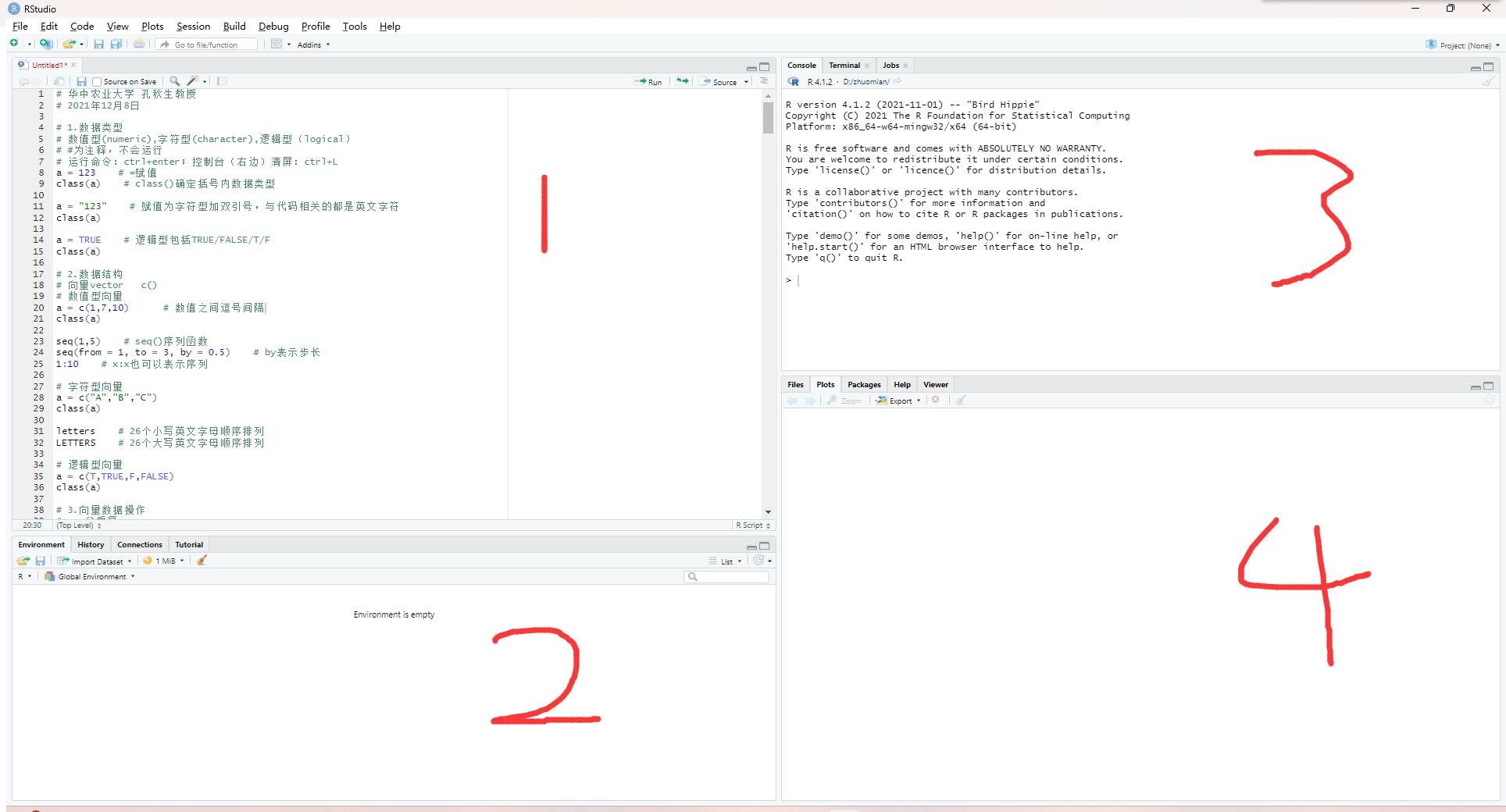
- Source窗口:写R代码的窗口,也可以在3窗口(console)写,个人习惯
- Environment、History等窗口:可以看到代码运行过程中生成的变量、自己的历史命令等等
- Console窗口:R语言的交互式控制台,可以逐行输入和执行R代码,并立即看到结果,ctrl+L可以清屏
- Files、Plot等窗口,前者可以看当前工作环境的文件,后者看到绘制的图
2和4窗口有多个选项供选择,我用的比较多的是这些,仅供参考。
对于1和3码代码的窗口部分,对于有较大代码块或者需要保存和重复的代码,建议用Source窗口,运行每一行需要Ctrl+回车;而对于简单的代码测试、快速计算或者做交互式探索的话,可以选择在Console窗口,回车就可以运行。
R语言要调用的软件包在CRAN仓库中,我们可以在以下R包官网中找到你需要的R包,以及各R包的参数、用法。
CRAN - Contributed Packages (r-project.org)
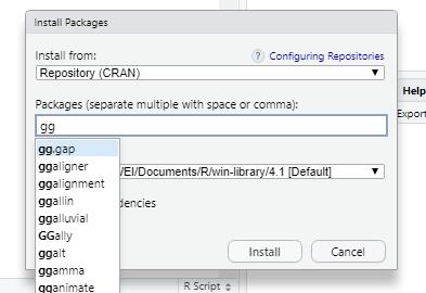
在Rstudio中,你可以通过菜单栏Tools,下拉框的第一个Install Packages窗口,输入你想要安装的R包,点击install安装:
以上是认识R和Rstudio的最基础的知识,下面主要讲讲R代码的语法和作图的一些示例。
3. R代码基础语法
再次申明这是入门写的笔记,不会介绍很详细,完整的可以看官方手册An Introduction to R (r-project.org)
为了方便展示运行结果,以下运行结果前均以两个井号##开头。
3.1 数据类型
常用的数据类型有数值型(numeric),字符型(character),逻辑型(logical)。
1 | a = 123 # =赋值,<-也可以赋值,R官方社区用<-较多,自己取舍。#表示注释,不会运行 |
3.2 数据结构
在R中,向量是一种基本的数据结构,用于存储一系列相同类型的元素。
1 | # 向量vector c()这个函数用来创建向量 |
3.3 向量数据操作
1 | # rep()重复 |
3.4 向量计算
1 | # +, -, *, / 加减乘除正常计算 |
3.5 向量类型转换
1 | # as.+数据类型() |
3.6 常用计算函数
1 | mean(1:10) # 平均数 |
3.7 矩阵(matrix)
矩阵是一种二维数据结构,由行和列组成,其中每个元素有相同的数据类型。矩阵可以看成是向量的拓展。
1 | # matrix(data = NA, nrow = 1, ncol = 1, byrow = FALSE, dimnames = NULL) |
3.8 数据框(Data Frame)
数据框是R语言中另一种常见的二维数据结构,它可以存储不同类型的数据,比如数值、字符、因子(factor)等等,并且每一列可以有不同的长度。
1 | data.frame(1:12,5:8) # 注意行数不同,填充方式不同 |
1 | ## 练习:生成一个矩阵,包含21-40的值,给行和列取名 |
4. R做图
咱们学生物最关心的就是怎么作图了,上面的编程基础没懂也没事,下面怎么画图可以套模板。
R可以导入不同的包作图,这里用最最基础的ggplot为例,以下是安装和导入方式,后面所有例子均需导入ggplot:
1 | # 安装ggplot2包 |
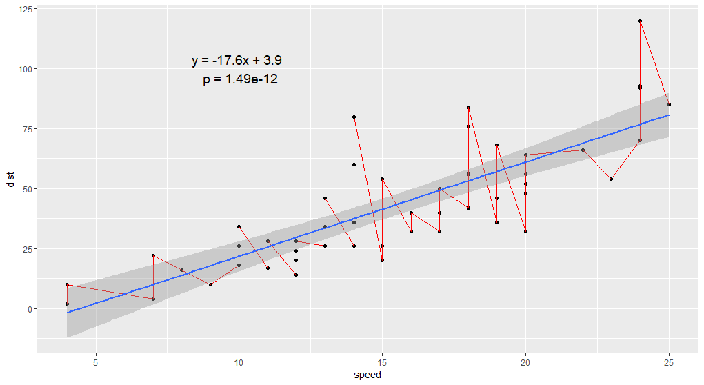
4.1 线性回归图
1 | library(ggplot2) |
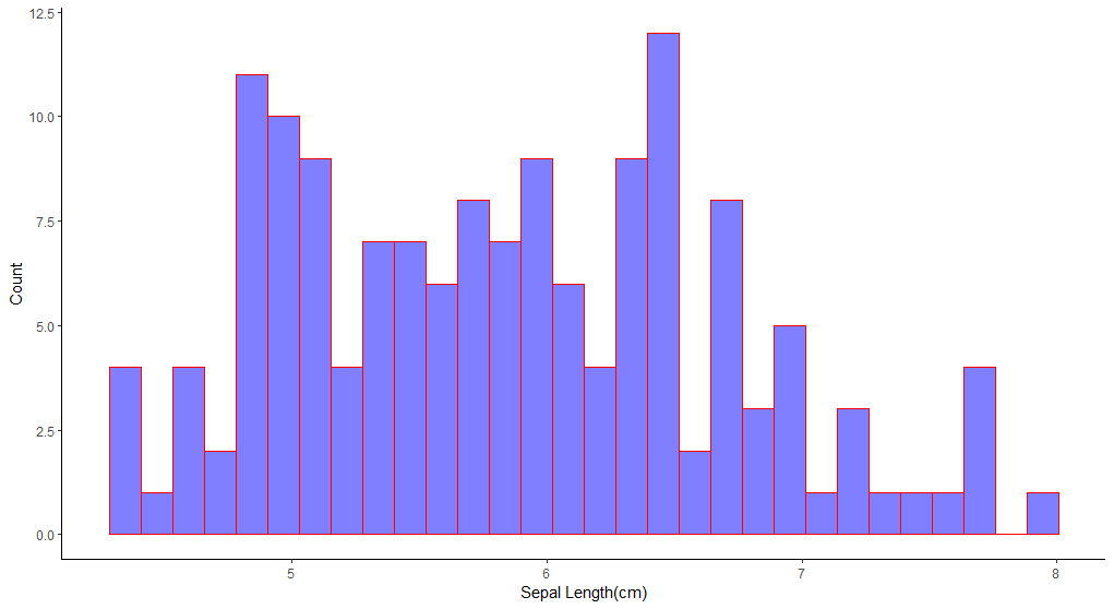
4.2 直方图
1 | library(ggplot2) |
4.3 密度图
1 | library(ggplot2) |
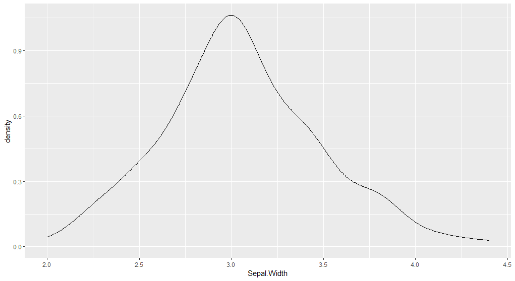
1 | # 密度图 + 直方图 |

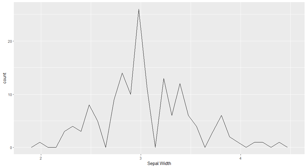
4.4 折线图
1 | library(ggplot2) |
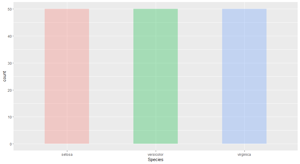
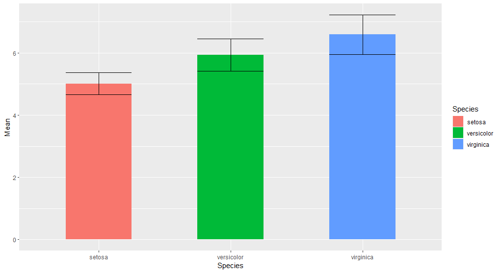
4.5 柱形图
1 | library(ggplot2) |
1 | # 柱形图叠加误差棒 |
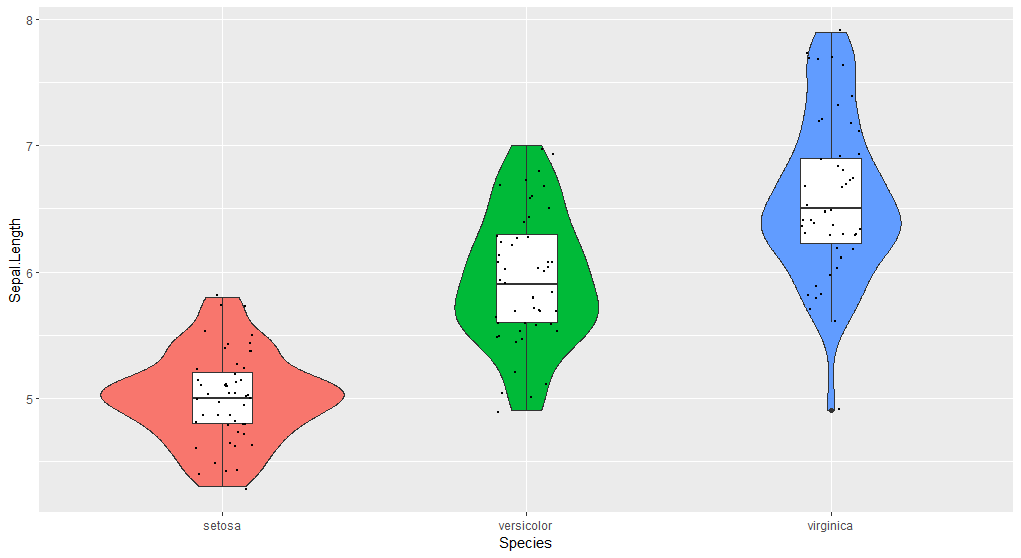
4.6 箱式图
1 | library(ggplot2) |
4.7 一些简单的练习
1 | ## 练习:以iris为例,做Sepal.Length和Petal.Length回归分析,并可视化 |

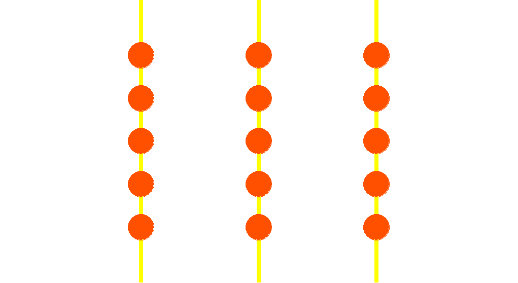
1 | ## 练习:做个糖葫芦? |
1 | ## 练习:做个字母表? |
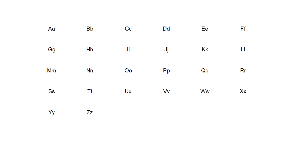
1 | ## 优化一下,做个炫彩字母表?大写字母在上,小写字母在下 |

1 | ## 算了 自由发挥吧,图就不放了 |